GPS_Regressor Tool (continuous treatments, continuous outcomes)
In this example, we use this package’s GPS_Regressor tool to estimate the marginal causal curve of some continuous treatment on a continuous outcome, accounting for some mild confounding effects. To put this differently, the result of this will be an estimate of the average of each individual’s dose-response to the treatment. To do this we calculate generalized propensity scores (GPS) to correct the treatment prediction of the outcome.
Compared with the package’s TMLE method, the GPS methods are more computationally efficient, better suited for large datasets, but produces wider confidence intervals.
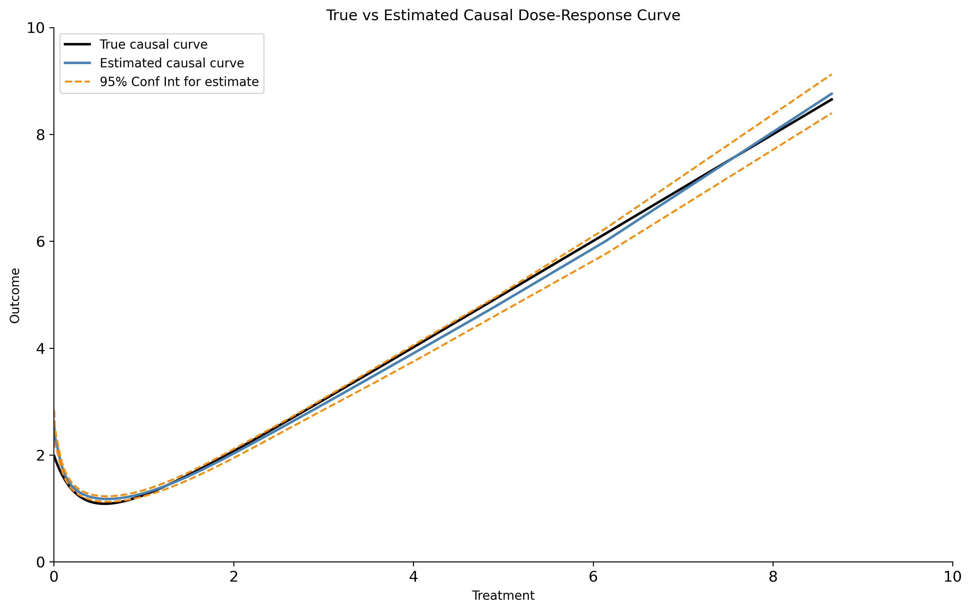
In this example we use simulated data originally developed by Hirano and Imbens but adapted by others (see references). The advantage of this simulated data is it allows us to compare the estimate we produce against the true, analytically-derived causal curve.
Let \(t_i\) be the treatment for the i-th unit, let \(x_1\) and \(x_2\) be the confounding covariates, and let \(y_i\) be the outcome measure. We assume that the covariates and treatment are exponentially-distributed, and the treatment variable is associated with the covariates in the following way:
>>> import numpy as np
>>> import pandas as pd
>>> from scipy.stats import expon
>>> np.random.seed(333)
>>> n = 5000
>>> x_1 = expon.rvs(size=n, scale = 1)
>>> x_2 = expon.rvs(size=n, scale = 1)
>>> treatment = expon.rvs(size=n, scale = (1/(x_1 + x_2)))
The GPS is given by
If we generate the outcome variable by summing the treatment and GPS, the true causal curve is derived analytically to be:
The following code completes the data generation:
>>> gps = ((x_1 + x_2) * np.exp(-(x_1 + x_2) * treatment))
>>> outcome = treatment + gps + np.random.normal(size = n, scale = 1)
>>> truth_func = lambda treatment: (treatment + (2/(1 + treatment)**3))
>>> vfunc = np.vectorize(truth_func)
>>> true_outcome = vfunc(treatment)
>>> df = pd.DataFrame(
>>>     {
>>>         'X_1': x_1,
>>>         'X_2': x_2,
>>>         'Treatment': treatment,
>>>         'GPS': gps,
>>>         'Outcome': outcome,
>>>         'True_outcome': true_outcome
>>>     }
>>> ).sort_values('Treatment', ascending = True)
With this dataframe, we can now calculate the GPS to estimate the causal relationship between treatment and outcome. Let’s use the default settings of the GPS_Regressor tool:
>>> from causal_curve import GPS_Regressor
>>> gps = GPS_Regressor()
>>> gps.fit(T = df['Treatment'], X = df[['X_1', 'X_2']], y = df['Outcome'])
>>> gps_results = gps.calculate_CDRC(0.95)
You now have everything to produce the following plot with matplotlib. In this example with only mild confounding, the GPS-calculated estimate of the true causal curve produces has approximately half the error of a simple LOESS estimate using only the treatment and the outcome.
The GPS_Regressor tool also allows you to estimate a specific set of points along the causal curve. Use the predict and predict_interval methods to produce a point estimate and prediction interval, respectively.
References
Galagate, D. Causal Inference with a Continuous Treatment and Outcome: Alternative Estimators for Parametric Dose-Response function with Applications. PhD thesis, 2016.
Moodie E and Stephens DA. Estimation of dose–response functions for longitudinal data using the generalised propensity score. In: Statistical Methods in Medical Research 21(2), 2010, pp.149–166.
Hirano K and Imbens GW. The propensity score with continuous treatments. In: Gelman A and Meng XL (eds) Applied bayesian modeling and causal inference from incomplete-data perspectives. Oxford, UK: Wiley, 2004, pp.73–84.